How can I trial BioVinci?
When downloading BioVinci software at https://vinci.bioturing.com/feature, users will automatically have 15 trial days.
Which features are restricted under the trial version?
Under the trial version, users can use full analytics and visualization features of BioVinci, but this version does not support export visualization results without the BioVinci watermark.
How can I purchase BioVinci?
You can find detail information about the price and purchase BioVinci on the website: https://vinci.bioturing.com/pricing
What types of input data are supported by BioVinci?
BioVinci supports for submitting these input data type: .vinci, .tsv, .csv, .xls, .xlsx, .feather file
Especially, .feather is a fast and reliable format for storing data in Python and R.
What types of files can be exported from BioVinci?
Users can export visualization results from editing plot features under .PNG or .SVG file without BioVinci watermark.
4.1.1. Normalization
Why do we need normalization?
BioVinci uses normalization for removing influences of confounding factors that lead to the differences among samples in input data. Normalization is the process of scaling individual samples to have unit norm.
How does normalization work?
Normalization calculates the norm of each sample (row vector) in the data and divides the value of each sample by its norm.
Step by step:
- Calculate the norm of each sample (row) in the data.
- Divide the value of each sample by its norm into the data.
We use the L2 norm as the default parameter and L1 norm as an optional parameter.
How does normalized data look like?
The normalized data have unit norm (L2) for each sample (row vector).
Input:
| 1 | -1 | 2 |
| 2 | 0 | 0 |
| 0 | 1 | -1 |
Output:
| 0.40 | -0.40 | 0.81 |
| 1 | 0 | 0 |
| 0 | 0.7 | -0.7 |
L2 norm of the first \(row (1, -1, 2) = \sqrt{1 + 1 + 4} = \sqrt{6}\). Hence, the
normalized vector has the following coordinates:
\({1 \over \sqrt{6}} = 0.40\)
\({-1 \over \sqrt{6}} = 0.40\)
\({2 \over \sqrt{6}} = 0.81\)
4.1.2. Standardization (mean removal and variance scaling)
Why do we need standardization?
Many machine learning algorithms assume that all features are centered around zero and have variance in the same order to avoid features with high variances can affect the accuracy of the estimated result. Standardization can be used when features have many different levels of variance.
How does standardization work?
Standardization involves calculating the mean u and the standard deviation s of each feature (column vector) and transforming the values in each column to \({{x-u} \over s}\).
Step by step:
- Calculate the mean u and standard deviation s of each feature (column vector) in the training data
- Transform the data by subtracting the mean and dividing the standard deviation for each feature: \(z = {{x - u} \over s}\).
How does standardized data look like?
Scaled training data has zero mean and unit variance.
Input:
| 0 | 0 |
| 0 | 0 |
| 1 | 1 |
| 1 | 1 |
Output:
| -1 | -1 |
| -1 | -1 |
| 1 | 1 |
| 1 | 1 |
The first feature of the data (first column): (0, 0, 1, 1)
\(Mean = {{0 + 0 + 1 + 1} \over 4} = 0.5\)
Standard deviation = 0.5
\(-1 = {{0 - 0.5} \over 0.5}\)
\(-1 = {{0 - 0.5} \over 0.5}\)
\(1 = {{1 - 0.5} \over 0.5}\)
\(1 = {{1 - 0.5} \over 0.5}\)
4.1.3. Normalization compared to Standardization
What is the difference between normalization and standardization?
Normalization calculates the norm of each sample (row vector) in the data and divides the value of each sample by its norm.
Meanwhile, standardization calculates the mean u and the standard deviation s of each feature (column vector) and transforms the values in each column to \({{x-u} \over s}\).
BioVinci 2.0 set normalization as a default parameter for preprocessing some types of data as single-cell RNA, bulk RNA, miRNA expression... For other data types, we suggest using standardization when features have many different levels of variance. On the other hand, if you like to remove the influences of confounding factors that lead to the differences among samples in your input data, the normalization is more suitable.
Reference: https://scikit-learn.org/stable/modules/preprocessing.html
How does standardization work?
Standardization involves calculating the mean u and the standard deviation s of each feature (column vector) and transforming the values in each column to \({{x-u} \over s}\).
Step by step:
- Calculate the mean u and standard deviation s of each feature (column vector) in the training data
- Transform the data by subtracting the mean and dividing the standard deviation for each feature: \(z = {{x - u} \over s}\).
How does standardized data look like?
Scaled training data has zero mean and unit variance.
Input:
| 0 | 0 |
| 0 | 0 |
| 1 | 1 |
| 1 | 1 |
Output:
| -1 | -1 |
| -1 | -1 |
| 1 | 1 |
| 1 | 1 |
The first feature of the data (first column): (0, 0, 1, 1)
\(Mean = {{0 + 0 + 1 + 1} \over 4} = 0.5\)
Standard deviation = 0.5
\(-1 = {{0 - 0.5} \over 0.5}\)
\(-1 = {{0 - 0.5} \over 0.5}\)
\(1 = {{1 - 0.5} \over 0.5}\)
\(1 = {{1 - 0.5} \over 0.5}\)
4.2.1. Application of dimensionality reduction
Why do we need dimensionality reduction in bioinformatics?
One challenge of bioinformatics is developing effective ways to analyze high dimensional data and find structures of the data. Dimensionality reduction methods are powerful tools for finding important features of input data and getting insights into our data. These methods can also help to visualize the high-dimensional data.
What are the criteria BioVinci chooses to compare the level of fitness with the label of the data?
BioVinci will suggest the fittest dimensionality reduction methods correspond to this label. The criteria we choose to compare the level of fitness with the label is the Silhouette score. Silhouette refers to a method of interpretation and validation of consistency within clusters of data. The silhouette value is a measure of how similar a sample is to its own cluster (cohesion) compared to other clusters (separation). The silhouette ranges from −1 to +1, where a high value indicates that the object is well matched to its own cluster and poorly matched to neighboring clusters. If most objects have a high value, then the clustering configuration is appropriate. If many points have a low or negative value, then the clustering configuration may have too many or too few clusters.
Reference: Wikipedia - Silhouette (clustering)
4.2.2. Linear dimensionality reduction
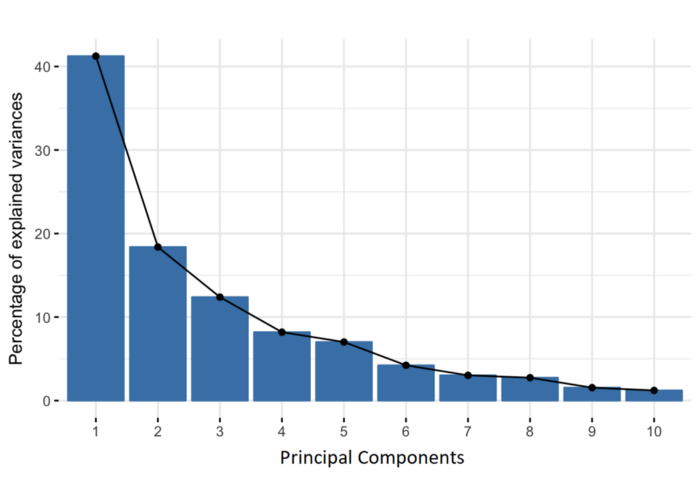
How does Principal Component Analysis (PCA) work?
Mathematically, PCA defines a new orthogonal coordinate system that optimally describes the variance in a dataset.
BioVinci uses sklearn.decomposition to do PCA by singular value decomposition (SVD). This method decomposes the input data X using SVD and computes sorted eigenvalues of the covariance matrix. In scikit-learn, PCA centers but does not scale the input data for each feature before applying the SVD.
Step by step:
- Centering input data.
-
Compute the covariance matrix.
The aim of this step is to understand how the variables of the input data set are varying from the mean with respect to each other, or in other words, to see if there is any relationship between them. Because sometimes, variables are highly correlated in such a way that they contain redundant information. -
Compute the eigenvectors and eigenvalues of the covariance matrix to identify the principal
components.
Eigenvectors and eigenvalues are the linear algebra concepts that we need to compute from the covariance matrix in order to determine the principal components of the data. Singular value decomposition can find eigenvectors and eigenvalues of the covariance matrix.
Principal component: Given a collection of points in two, three, or higher-dimensional space, a "best fitting" line can be defined as one that minimizes the average squared distance from a point to the line. The next best-fitting line can be similarly chosen from directions perpendicular to the first. Repeating this process yields an orthogonal basis in which different individual dimensions of the data are uncorrelated. These basis vectors are called principal components, and several related procedures principal component analysis (PCA).
Reference:
https://builtin.com/data-science/step-step-explanation-principal-component-analysis
https://scikit-learn.org/stable/modules/decomposition.html#pca
What are the differences between SVD solver options?
BioVinci uses sklearn.decomposition.PCA for implementing principal components analysis. There are some
differences between SVD solver options:
X is input data. The default parameter of SVD solver is “auto”.
Auto: If the input data is larger than 500x500 and the number of components to extract is lower than 80% of the smallest dimension of the data, then the more efficient ‘randomized’ method is enabled. Otherwise the exact full SVD is computed and optionally truncated afterwards.
Full: Run exact full SVD calling the standard LAPACK solver via scipy.linalg.svd and select the
components by postprocessing. More information about LAPACK here:
http://www.netlib.org/lapack/
Arpack: Run SVD truncated to n_components calling ARPACK solver via scipy.sparse.linalg.svds. It requires strictly 0 < n_components < min(n_sample of X, n_feature of X). More information about APPACK: https://www.caam.rice.edu/software/ARPACK/
Randomized: Run randomized SVD by the method of Halko et al, 2009. This paper presents a modular framework for constructing randomized algorithms that compute partial matrix decompositions. These methods use random sampling to identify a subspace that captures most of the action of a matrix. The input matrix is then compressed - either explicitly or implicitly - to this subspace, and the reduced matrix is manipulated deterministically to obtain the desired low-rank factorization. In many cases, this approach beats its classical competitors in terms of accuracy, speed, and robustness.
Reference:
https://arxiv.org/pdf/0909.4061.pdf
https://scikit-learn.org/stable/modules/generated/sklearn.decomposition.PCA.html
4.2.3. Non-linear dimensionality reduction
Why do we need non-linear dimensionality reduction?
The geodesic distances (shortest path) of two points can be different from their straight-line Euclidean distance in high-dimensional input space. The geodesic distances reflect the true low-dimensional geometry of the manifold, but some linear dimensionality reduction methods as PCA and MDS effectively see just the Euclidean structure; thus, they fail to detect the intrinsic distance (Tenenbaum et al., 2000). So this is the reason we integrated non-linear dimension reduction algorithms into our application.
How does (t-distributed Stochastic Neighbor Embedding) t-SNE work?
The t-SNE algorithm calculates a similarity measure between all pairs of instances in the high dimensional space and in the low dimensional space. It then tries to optimize these two similarity measures using a cost function. Conditional probabilities that represent similarities.
Step by step:
- Measure similarities between points in the high dimensional space. For each data point \(x_i\) center a Gaussian distribution over that point. Measure the density of all points \(x_j\) under that Gaussian distribution. This gives us a set of probabilities \(P_{ij}\) for all points. Those probabilities are proportional to the similarities. \(P_{ij} = {{P(i|j) + P(j|i)} \over 2N}\), where \(P(i|j)\) is the probability of \(x_i\) picking \(x_j\) as a neighbor. Where \(N\) is the number of data points.
- Instead of using a Gaussian distribution, use a Student t-distribution with one degree of freedom. This gives us a second set of probabilities \(Q_{ij}\) in the low dimensional space.
- Measure the difference between the probability distributions of the two-dimensional spaces using Kullback-Liebler divergence (KL). The larger the KL divergence value is, the more the difference between P and Q. Use gradient descent to minimize our KL cost function.
Reference:
http://www.jmlr.org/papers/volume9/vandermaaten08a/vandermaaten08a.pdf
https://towardsdatascience.com/an-introduction-to-t-sne-with-python-example-5a3a293108d1
What are the parameters of t-SNE?
Perplexity: is effectively the number of nearest neighbors when constructing the graph. Larger perplexities lead to more nearest neighbors and less sensitive to the small structures. Conversely, lower perplexities consider a smaller number of neighbors and thus ignore more global information in favor of the local neighborhood. As dataset sizes get larger, more points will be required to get a reasonable sample of the local neighborhood, and hence larger perplexities may be required. Similarly, noisier datasets will require larger perplexity values to encompass enough local neighbors to see beyond the background noise.
Early exaggeration factor: During the early exaggeration, the joint probabilities in the original space will be artificially increased by multiplication with a given factor. Larger factors result in larger gaps between natural clusters in the data. If the factor is too high, the KL divergence could increase during this phase.
Learning rate: If it is too low, gradient descent will get stuck in a bad local minimum. If it is too high, the KL divergence will increase during optimization.
The maximum number of iterations
Angle (not used in the exact method): Larger angles imply that we can approximate larger regions by a single point, leading to better speed but less accurate results.
How does ISOMAP work?
Isomap is used for computing a quasi-isometric, low-dimensional embedding of a set of high-dimensional data points. Quasi-isometry is a function between two metric spaces. ISOMAP constructs a neighborhood graph and computes the shortest path between two nodes in this graph. This is a k-neighbour based graph learning algorithm.
A high-level description of the ISOMAP algorithm:
-
Determine the neighbors of each point.
- All points in some fixed radius.
- K nearest neighbors.
-
Construct a neighborhood graph.
- Each point is connected to others if it is a k-nearest neighbor.
- Edge length equal to Euclidean distance.
-
Compute the shortest path between two nodes.
- Dijkstra's algorithm
- Floyd–Warshall algorithm
-
Compute lower-dimensional embedding.
- Multidimensional scaling: Multidimensional scaling (MDS) seeks a low-dimensional representation of the data in which the distances respect well the distances in the original high-dimensional space. In general, MDS is a technique used for analyzing similarity or dissimilarity data.
How does UMAP work?
From a theoretical perspective, UMAP finds the best low dimensional representation to have a similar fuzzy topological structure of high dimensional input space. From a practical computational perspective, UMAP can be described as a graph problem. As with other k-neighbor graph-based algorithms, UMAP can be described in two phases. In the first phase, a particular weighted k-neighbor graph is constructed. In the second phase, a low dimensional layout of this graph is computed.
Reference:
https://arxiv.org/pdf/1802.03426.pdf
What is the difference between ISOMAP and UMAP?
ISOMAP was built on classical MDS but it preserves the intrinsic geometry of the data, as captured in the geodesic manifold distances between all pairs of data points. We use ISOMAP as a non-linear method that is closest to linear dimension reduction methods.
Meanwhile, UMAP is a novel and powerful non-linear dimension reduction method.
From a practical computational perspective, UMAP can be described as a graph problem. In particular, it belongs to the class of k-neighbour based graph learning algorithms such as Laplacian Eigenmaps, Isomap, and t-SNE. The differences between all algorithms in this class amount to specific details in how the graph is constructed and how the layout is computed (McInnes et al., 2018).
What is the difference between tSNE and UMAP?
The most important difference between UMAP and t-SNE is the how-to compute the loss function.
Reference:
https://arxiv.org/pdf/1802.03426.pdf
What does the decision tree model do?
The decision tree model is used to define important features that distinguish a cluster from the whole of the population.
What is the difference between the Gini and entropy?
These are criteria as the function to measure the quality of a split. Supported criteria are “Gini” for the Gini impurity and “entropy” for the information gain.
Gini impurity:
The Gini impurity measure is one of the methods used in decision tree algorithms to decide the optimal
split from a node. Gini Impurity tells us what is the probability of misclassifying an observation. The
lower the Gini the better the split. In other words the lower the likelihood of misclassification.
\(G(k) = \sum{P(i)} * (1 - P(i))\) where \(P(i)\) is the probability of certain classification i, per the data set.
Information gain:
In information theory, the entropy can be interpreted as the average level of "information" or
"uncertainty" inherent in the variable's possible outcomes. Given a random variable X, with possible
outcomes x_i:$$H(X)=-\sum_{i=1}^n p(x_i)logp(x_i)$$
The conditional entropy (or equivocation) quantifies the amount of information needed to describe the outcome of a random variable Y given that the value of another random variable X is known.
In general terms, the expected information gain is the change in information entropy Η from a prior state to a state that takes some information as given: $$IG(T,a)=H(T) - H(T|a)$$ where \(H(T|a)\) is the conditional entropy of \(T\) given the value of attribute \(a\).
In the decision tree model, information gain of change state from a parent node to all its children is a criterion for splitting.
Gini impurity and information gain can make different splitting in the decision tree model, you can compare the results and choose your suitable criteria for your dataset.
Reference:
https://towardsdatascience.com/gini-impurity-measure-dbd3878ead33
https://en.wikipedia.org/wiki/Decision_tree_learning#Gini_impurity
How can I become a partner of BioVinci?
To bring the latest advancements in computer science and mathematics to life science, we can not work alone. BioVinci is open to partner with leading research institutions. If you want to adopt BioVinci in your research institute, please send us an email at vinci@bioturing.com.
References
Cluster analysis (clustering): is the task of grouping a set of objects in such a way that objects in the same group (called a cluster) are more similar (in some sense) to each other than to those in other groups (clusters).
A ranking: is a relationship between a set of items such that, for any two items, the first is either 'ranked higher than', 'ranked lower than' or 'ranked equal to' the second.
Principal component analysis: Given a collection of points in two, three, or higher-dimensional space, a "best fitting" line can be defined as one that minimizes the average squared distance from a point to the line. The next best-fitting line can be similarly chosen from directions perpendicular to the first. Repeating this process yields an orthogonal basis in which different individual dimensions of the data are uncorrelated. These basis vectors are called principal components, and several related procedures principal component analysis (PCA).
PCA is also related to canonical correlation analysis (CCA). CCA defines coordinate systems that optimally describe the cross-covariance between two datasets while PCA defines a new orthogonal coordinate system that optimally describes the variance in a single dataset.
https://en.wikipedia.org/wiki/Principal_component_analysis
Singular value decomposition: is a factorization of a real or complex matrix.
https://math.mit.edu/classes/18.095/2016IAP/lec2/SVD_Notes.pdf
http://www2.imm.dtu.dk/pubdb/edoc/imm4000.pdf
https://www.cc.gatech.edu/~lsong/teaching/CX4240spring16/pca_wall.pdf
https://en.wikipedia.org/wiki/Singular_value_decomposition
Correlation or dependence: is any statistical relationship, whether causal or not, between two random variables or bivariate data.
Classification: is the problem of identifying to which of a set of categories (sub-populations) a new observation belongs, on the basis of a training set of data containing observations (or instances) whose category membership is known.
Kernel method: is a class of algorithms for pattern analysis, whose best-known member is the support vector machine (SVM). The general task of pattern analysis is to find and study general types of relations (for example clusters, rankings, principal components, correlations, classifications) in datasets.